
Bayes Theorem for lawyers - Part 2: the 'odds' form and the Prosecutor's Difficulty
A mid-length explanation of the Ultimate Guide to the power of evidence

Recap
In Part 1 I used a criminal law example to explain the “probability form” of Bayes’ theorem. That was six months ago, absurdly, so first a very brief recap.
We saw that the effect a piece of evidence has on a hypothesis can be described by the mathematical relationships of two overlapping areas.
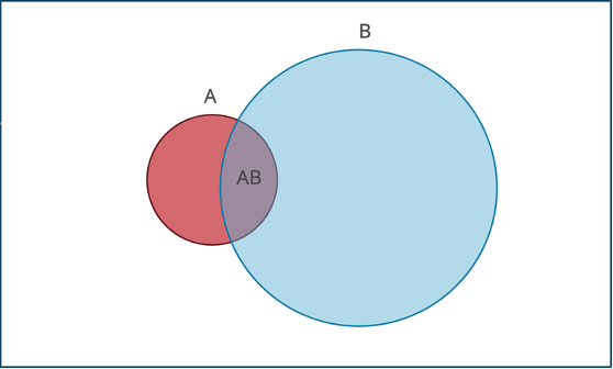
The size of the overlap AB can be described as either AB/B x B, or AB/A x A.
So AB/A x A = AB/B x B.
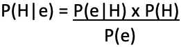
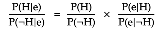
Intuitively, P(A|B) – that is, the probability of A given B – is AB/B. And likewise P(B|A) = AB/A. Substituting and rearranging gave us Bayes’ theorem (using H for hypothesis and e for evidence):
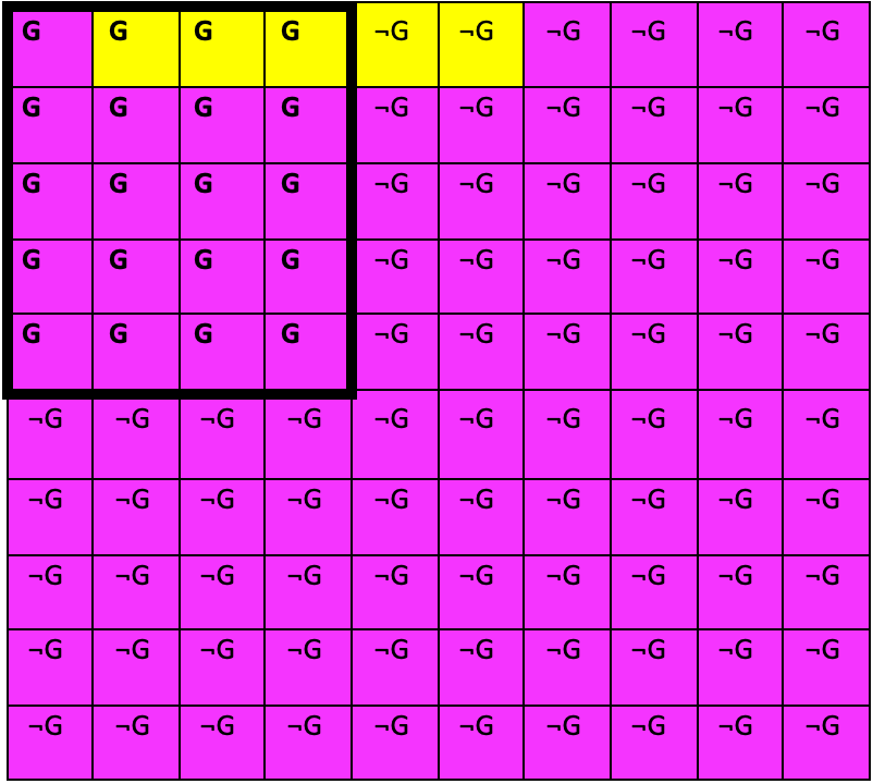
We worked through a criminal law example. An island of 100 inhabitants. 20 rioters. Every islander rides a motorbike. 25 Yamahas on the island, 75 made by other manufacturers. Of the rioters, 15 ride Yamahas.
Putting this information into a diagram like Fig. 1 gave us this

the overlapping areas being: the dark-outlined rectangle top left which contains the G squares (which represents the prior probability of our hypothesis, H), and the yellow area (which represents the probability of our evidence, e). The ¬ symbol means “not”.
The probability that a randomly selected inhabitant was a rioter was 0.20. But when the police discovered he rode a Yamaha, we calculated an updated probability of guilt, P(H|e), which was 0.60, using the Bayes equation.
Odds form
We then noted that what matters is the ratio of Yamahas-among-the-guilty to Yamahas-among-the-innocent – or to use proper notation, the ratio of P(e|H) : P(e|¬H), which is known as the ‘likelihood ratio’. It is this ratio, rather than the absolute values of P(e), P(e|H), or P(e|¬H), that determines probative power.
If we change the numbers so that our diagram looks like this,
then the new evidence – i.e. the police’s discovery that the man is a Yamaha rider – would have exactly the same effect on P(H) as it did when the numbers were as in Fig. 4: in both cases, the chance of guilt starts at 0.20, and the new evidence raises it to 0.60. This is because the ratio (15/20 : 10/80) is the same as (3/20 : 2/80), i.e. 6 to 1. Or to write the ratios as fractions: (15/20) / (10/80) = (3/20) / (2/80) = 6.
Now, using a likelihood ratio, P(e|H) : P(e|¬H), to update the probability of a hypothesis is usually easier than using the probability form of the Bayes equation. For one thing, you don’t have to find P(e), the "probability of the evidence”. P(e) can be a confusing concept, and hard to estimate a value for in many real-world scenarios.
So, first you have to convert P(H) into odds. If P(H) = 0.20, as in the rioters example, the odds will be 0.20 : 0.80 = 1 : 4. You then simply multiply these odds by the likelihood ratio to get the updated odds:
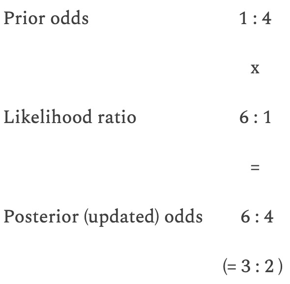
The posterior odds can of course easily be converted back to a probability: 3/(3+2) = 0.60, or 60%.
It is best if we write the ratios as fractions:
To be clear: this so-called “odds form” of the Bayes equation is not much more than a re-arrangement of the probability form. The re-arrangement is explained neatly here1.
Conceptually, the odds form is preferable because it focusses the mind on what matters: a comparison between the likelihood of the evidence if the defendant is guilty, and the likelihood of the evidence if the defendant is innocent.
Practically, the odds form is preferable because it is easier to use, particularly if we want to assess the combined effect of several different bits of evidence, as we do in court: likelihood ratios can just be multiplied together.
The Prosecutor’s Difficulty
For instance, imagine that in our rioters example, after the motorbike evidence we discover that 90% of the rioters were male (like our suspect), against a background of 50% in the general population. This gives a likelihood ratio of 9/4 (because 90% of the rioters is 18 men, which leaves 32 among the 80 innocent islanders, which is 40%).
And then imagine we discover (somehow) that half the rioters fled to their homes in the North of the island, the other half to their homes in the South – and we find that only 24% of islanders live South, including our suspect. This gives a likelihood ratio of 22/7 (among the guilty, 1/2 live South; among the innocent, 14/80; (1/2) / (14/80) = 22/7).
To calculate the effect of these three separate pieces of evidence, we can simply multiply the prior odds by each of the likelihood ratios:
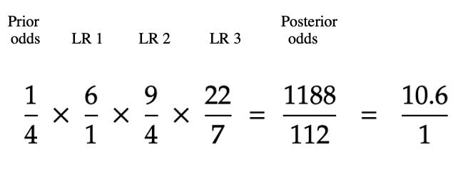
Those odds, 10.6 : 1, are equivalent to a probability of guilt of 91%.
Which illustrates an important point – one that prosecutors, I think, struggle to sell to juries, and indeed judges.
Weak evidence quickly adds up – or, rather, multiplies up – to powerful evidence.
91% is clearly short of what is required for conviction – “sure”, or in the old formulation, “beyond reasonable doubt”. But two more pieces of evidence with likelihood ratios of 4 : 1 would raise it to over 99%.
Consider the first bit of evidence, the motorbikes. Looking again at Fig. 4, it’s intuitively clear that Yamahas are significantly over-represented among the guilty. And the likelihood ratio of that evidence, 6 : 1, is decent. But if the Crown tried to claim it was “very powerful” evidence, and invited the jury to rely on it heavily, the defence would object that there are plenty of innocent Yamaha riders who the defendant could be. They might say that the evidence “doesn’t prove anything” and that it is “entirely consistent with innocence”. And they would be right.
As for the other two pieces of evidence, the Crown risks derision. “The prosecutor asks you to convict,” the defence might say, “on the basis that the defendant is a man – when men make up a full 40% of innocent islanders! This tells you one thing: they have a weak case, and are clutching at straws.”
And yes, on its own, 9/4 is weak stuff. But it only takes eight pieces of evidence with a likelihood ratio of 9/4 to raise a 20% prior probability of guilt to a posterior probability of over 99%. This is not in line with our intuitions.
So what can a prosecutor do? Explaining Bayes’ theorem to a jury is out of the question. But an analogy with an accumulator bet on the horses, in a speech? I think that would be fair, and sometimes effective.
But their best bet might be to follow what I feel is common practice: only bring cases that have at least one piece of stand-alone very strong evidence, and don’t lean too heavily on the rest.
Using Bayes in practice
I have found that to assess the strength of a piece of evidence, and to formulate arguments for the jury one way or the other, it is sometimes useful to do two things. First, draw a roughly-to-scale diagram of the two overlapping areas, P(H) and P(e), like Fig. 4, and describe what each of the four separate areas (H and e, H and ¬e, ¬H and e, ¬H and ¬e) really means for the particular evidential scenario in hand.
And secondly, and separately, try to estimate the likelihood ratio by asking ‘how likely would this evidence be if the defendant was guilty, compared to its likelihood if he was innocent?’
Bayes theorem took me a while to understand properly - and of course my understanding is not complete. I don’t think I would have fully ‘got it’ from any single source on its own, so as promised in Part 1, here is are some links to some explanations I found particularly helpful.
A very nice, short graphical illustration from 2009 by Oscar Carbonilla.
Eliezer Yudkowsky’s 2003 explainer. Long and slow. Very widely read.
A 2010 post by Luke Muehlhauser, referencing and lightly criticising Yudkowsky’s tutorial. Also long and slow.
A short illustration by the innovative means of Venn pie charts! Not to everyone’s tastes, but I found it very useful.
A tutorial from Professor Norman Fenton’s blog. Focusses on criminal law. Extremely concise.
The Arbital collection of explanations. A choice of ‘speeds’. A bit messy to navigate, but much of it very good.
If you want to work through that explanation of how to derive the odds form from the probability form, I would add the following tip. “P(¬G|e) x P(e) = P(e|¬G) x P(¬G)”: this becomes intuitively clear when you see that the two sides of that equation are just two different ways of describing the size of the area “e and ¬G”, or to use the rioters example, the proportion of innocent Yamaha riders on the island. See my Fig. 4.
Super interesting!
Great explainer!